EDO non linéaire

import numpy as np
import matplotlib.pyplot as plt

f = lambda x, t: t * np.sin(x)

def euler(f, x0, t0, tf, n):
    h = (tf - t0) / n
    t = np.linspace(t0, tf, n+1)
    x = np.zeros(n+1)
    x[0] = x0
    for k in range(n):
        x[k+1] = x[k] + h * f(x[k], t[k])
    return t, x

def rk2_heun(f, x0, t0, tf, n):
    h = (tf - t0) / n
    t = np.linspace(t0, tf, n+1)
    x = np.zeros(n+1)
    x[0] = x0
    for k in range(n):
        k1 = f(x[k], t[k])
        k2 = f(x[k] + h * k1, t[k] + h)
        x[k+1] = x[k] + (h/2) * (k1 + k2)
    return t, x

def rk4(f, x0, t0, tf, n):
    h = (tf - t0) / n
    t = np.linspace(t0, tf, n+1)
    x = np.zeros(n+1)
    x[0] = x0
    for k in range(n):
        k1 = f(x[k], t[k])
        k2 = f(x[k] + 0.5*h*k1, t[k] + 0.5*h)
        k3 = f(x[k] + 0.5*h*k2, t[k] + 0.5*h)
        k4 = f(x[k] + h*k3, t[k] + h)
        x[k+1] = x[k] + (h/6)*(k1 + 2*k2 + 2*k3 + k4)
    return t, x

# Paramètres
x0 = 1.0
t0, tf = 0.0, 5.0
n = 50 # h = 0.1

t_euler, x_euler = euler(f, x0, t0, tf, n)
t_rk2, x_rk2 = rk2_heun(f, x0, t0, tf, n)
t_rk4, x_rk4 = rk4(f, x0, t0, tf, n)

plt.figure(figsize=(10, 6))
plt.plot(t_euler, x_euler, 'r-', label='Euler (ordre 1)')
plt.plot(t_rk2, x_rk2, 'g-', label='RK2 Heun (ordre 2)')
plt.plot(t_rk4, x_rk4, 'b-', label='RK4 (ordre 4)')
plt.xlabel('t')
plt.ylabel('x(t)')
plt.title('Comparaison des méthodes')
plt.legend()
plt.grid(True, alpha=0.3)
plt.show()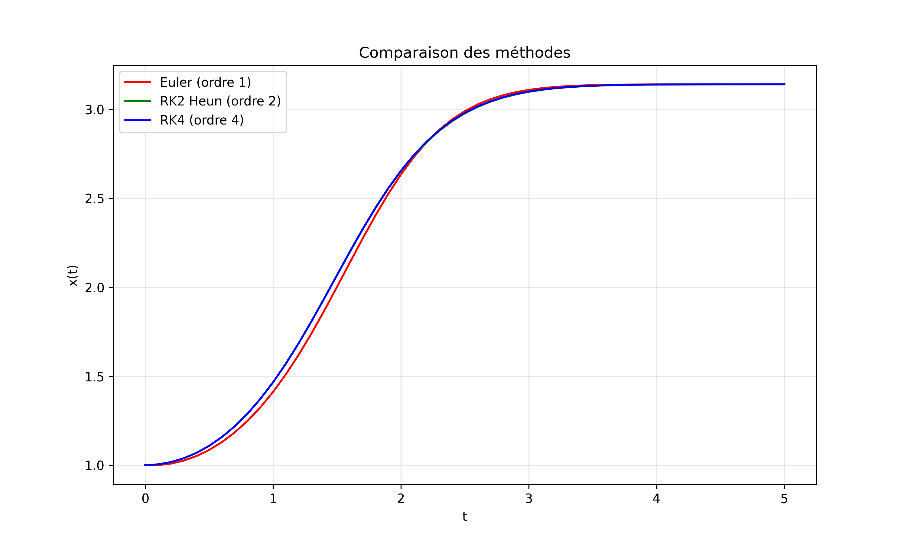

Résolution de $x^{\prime }=t\sin (x)$ par Euler, RK2 (Heun), et RK4.

La courbe RK4 est la plus précise et converge de manière stable, tandis qu'Euler montre des oscillations de pas.